Mia Tadic
DATA ENGINEER
We are talking about what is HPC, the motivation to use it, and then we choose the world of Slurm to test the performances of one specific HPC cluster.
This blog post is conceived as an intro in high performance computing, not from a scientific point of view, but a user’s perspective. We are talking about what is HPC, the motivation to use it, and then we choose the world of Slurm to test the performances of one specific HPC cluster. We will describe the cluster setup on GCP and train a Keras machine learning model on a distributed dataset of images using TensorFlow and Python. Spoiler alert: keep along to see the satisfactory time gain results!
What is HPC?
High Performance Computing (HPC) is the use of supercomputers and parallel processing techniques for solving complex computational problems.
HPC technology focuses on developing parallel processing algorithms and systems by incorporating both administration and parallel computational techniques.
HPC is typically used for solving advanced problems that require a lot of time.
Why HPC?
When you have loads of data and its processing takes a really long time, the approachdivide et imperacomes to hand.
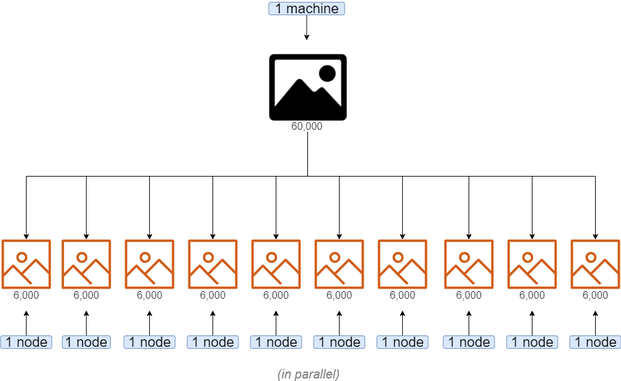
With HPC, you can divide your job so that every node processes different partitions of the data in parallel, speeding up the execution time.
For example, let’s look at the use case of analyzing and classifying large dataset of images. In advanced use cases, it would take a serious amount of time (hours, maybe even days) to complete the process.
Using HPC, you can divide the dataset into several partitions and manage several nodes to process one batch of images each. So, if your job needed 20 hours to process all the images, use multiple nodes to complete the job in e.g. 2 hours.
Slurm and GCP
Slurm is one of the leading workload managers for HPC clusters around the world. Slurm provides an open-source, fault-tolerant, and highly-scalable workload management and job scheduling system for small and large Linux clusters. Slurm requires no kernel modifications for its operation and is relatively self-contained. As a cluster workload manager, Slurm has three key functions:
-
It allocates exclusive or non-exclusive access to resources (compute nodes) to users for some duration of time so they can perform work.
-
It provides a framework for starting, executing, and monitoring work (normally a parallel job) on the set of allocated nodes.
-
It arbitrates contention for resources by managing a queue of pending work.
To make it easier all together, Google and SchedMD (Slurm’s creators) joined forces and as a result, you can run a Slurm cluster on Google Cloud Platform! You do not have to worry about all those parallel techniques since Slurm takes care of that (you just name the parameters you like) and GCP takes care of the setting up a cluster and providing resources.
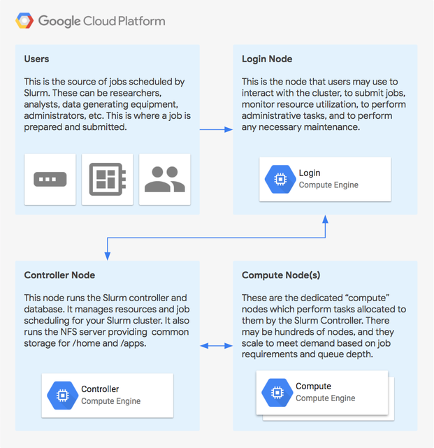
Basic architectural diagram of a stand-alone Slurm Cluster in Google Cloud Platform:
As can be seen in the picture above, Slurm cluster contains three types of nodes:login, controller,andcompute node.
-
Login node serves as an interface for the user: the user should communicate with the cluster exclusively through the login node (starting the job, requiring resources, …)
-
Controller node manages resources and job scheduling for the user (intuitively, in distributed world’s terminology, it acts as amaster)
-
Compute nodes execute the job (intuitively, in distributed world’s terminology, they act asslaves)
Setting Up a Slurm Cluster on GCP
Before describing the setup, let us explain in short how does GCP implement a Slurm cluster.
In GCP, a cluster is realized as a deployment. A deployment is an instantiation of a set of resources that are defined in a configuration. A deployment can contain a number of resources, across a variety of Google Cloud Platform services. When you create a deployment, Deployment Manager creates all of the described resources in the respective Google Cloud Platform APIs.
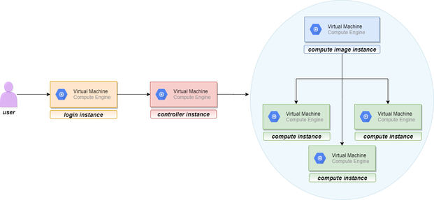
This brings us to the cluster’s nodes. Each node in a cluster is actually a virtual machine – a GCP resource. When a deployment is created, three new virtual machines appear in ”VM instances” page, under “Compute Engine“. Those VMs arelogin instance, controller instance,andcompute image instance.
Compute instances require a bit more attention. One thing to notice is that deployment does not create compute instance, but computeimageinstance. The second thing to notice is that it creates exactly one compute image instance, even if you request more compute nodes in your cluster. So, if a user requests 10 compute nodes for the cluster, those 10 virtual machines will not be immediately instantiated with the cluster deployment. Here’s what is happening. These compute instances are created in the later step when you run a job and request the number of nodes for the job. Then the compute nodes will be allocated, and they will appear in the ”VM instances” page. Shortly after the job is completed (whether successfully or not), these virtual machines will be deallocated and will disappear from the list. This way, a user gets new compute VMs every time. Now, why is the computeimagehere? Computeimageserves as a template for the compute instances that will be dynamically allocated. So, this compute image is present all the time, waiting for the job to request the nodes, and then thecontrollernode will allocate new compute VMs based on compute image VM.
And here is the visual representation of the described process:
Finally, let’s head to the cluster setup. In this blog post, we will run distributed training on a cluster that contains 10computenodes. Customize the information so that they suit your needs:
- Launch Google Cloud Shell.
- Check that you already authenticated and that the project is already set to yourPROJECT_ID:
$ gcloud auth list Credentialed accounts: @.com (active) $ gcloud config list project [core] project = <PROJECT_ID> - Clone git repository that contains the Slurm for Google Cloud Platform deployment-manager files:
git clone https://github.com/SchedMD/slurm-gcp.git
- Switch to the Slurm deployment configuration directory:
cd slurm-gcp - Configure the Slurm Deployment YAML file. Provide information that suits your needs. There are plenty more parameters available, they can be found in
SchedMD’s GitHub repository. Below is the script that was sufficient for our needs.#[START cluster_yaml] imports: – path: slurm.jinja resources: – name:
slurm-cluster type: slurm.jinja properties: cluster_name : slurm10 zone :
europe-west4-a controller_machine_type : n1-standard-2
login_machine_type : n1-standard-2 compute_image_machine_type :
n1-standard-2 default_users : partitions : – name : debug machine_type :
n1-standard-2 max_node_count : 10 zone : europe-west4-a - In the Cloud Shell session, execute the following command from the
slurm-gcpfolder:1gcloud deployment-manager deployments create slurm-deployment --config slurm-cluster.yamlThis command creates a deployment named slurm-deployment. The operation can take a few minutes to complete, so please be patient. - Verify the deployment (Navigation menu →
Deployment Manager) - Verify the cluster’s instances (Navigation menu →
Compute Engine) – there should belogin,controller,andcompute imageinstances.Computeinstance(s) show up only when you allocate them for the sbatch job. They disappear shortly after the job is completed - Log in tologininstance (Navigation menu → Compute Engine→SSH button next to thelogininstance).
Note:If the following message appears upon login:
*** Slurm is currently being installed/configured in the background. ***
A terminal broadcast will announce when installation and configuration is complete.
/home on the controller will be mounted over the existing /home.
Any changes in /home will be hidden. Please wait until the installation is complete before making changes in your home directory.
Do not proceed with the lab until you see this message (approximately 5 mins):
*** Slurm logindaemon installation complete ***
/home on the controller was mounted over the existing /home.
Either log out and log back in or cd into ~.
Once you see this message please log out and log back into logininstance to continue the work.
Testing: Image Classification with Machine Learning
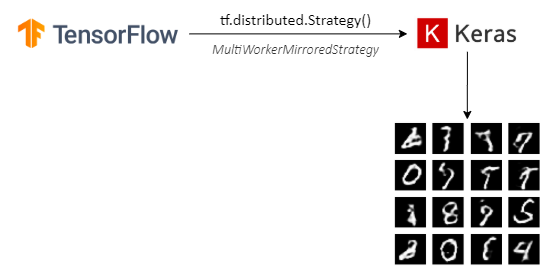
The example that will be shown in this blog post is a Keras machine learning model that classifies 60,000 MNIST images of handwritten digits. It is a simple convolutional neural network algorithm.
Now, there is a specific problem to address while incorporating distribution in the machine learning model. In ML models, there are some variables that must be shared among the nodes and all the nodes must update those very same variables (e.g. the gradient or the weights). Otherwise, if every node calculates its own gradient or updates its own weights, you would effectively end up with different models on each node. So, the nodes must communicate somehow. We can use some API that enables the communication and usage of the same variables across the nodes. In this blog post, we will use TensorFlow’s tf.distribute.Strategy API, and integrate it with the mentioned Keras model.
As described thoroughly in TensorFlow’s official pages, tf.distribute.Strategy is a TensorFlow API to distribute training across multiple GPUs, multiple machines or TPUs. In this blog post, we show the synchronous distributing training with data parallelism across multiple machines (compute nodes), usingMultiWorkerMirroredStrategyand following TensorFlow’s official tutorial. The training will be executed on nodes’ CPUs.
This strategy creates copies of all variables in the model on each device across all machines. It uses CollectiveOps as the multi-worker all-reduce communication method used to keep variables in sync.
One of the key differences to get multi worker training going, as compared to (multi-GPU) training on one machine, is the multi-worker setup. TheTF_CONFIGenvironment variable is the standard way in TensorFlow to specify the cluster configuration to each worker that is part of the cluster.
REQUIREMENTS
Although TensorFlow suggests its latest version (at the time of writing) 2.0.1, we could not get the code running with it. So, we will describe the environment that suited us.
-
SSH tologininstance in your Slurm cluster and obey all of the steps from there.
-
Installing Python version 3.7.4 in /home:
-
Install Python:
$ cd ~ $ mkdir tmp $ cd tmp $ wget
https://www.python.org/ftp/python/3.7.4/Python-3.7.4.tgz $ tar zxvf
Python-3.7.4.tgz $ cd Python-3.7.4 $ ./configure
--prefix=$HOME/opt/python-3.7.4 $ make $ make install
-
Use the new version of Python over the system default:
$ cd ~ $ vi ~/.bash_profile (add line: export PATH=$HOME/opt/python-3.7.4/bin:$PATH) $ . ~/.bash_profile
-
Check the new version:
$ which python3 (output should be: /home//opt/python-3.7.4/bin/python3) $ python --version (output should be: Python 3.7.4)
Note: We intentionally installed Python in /home directory, even though /usr would be more common and correct. The reason is that only /home and /apps are shared directories across all instances in Slurm cluster. So, if you install something in /usr folder fromlogininstance,computeinstances (i.e. the worker instances that actually run the code) will not see it.
3. Installing and creating a virtual environment:
-
Install virtualenv:
$ curl https://bootstrap.pypa.io/get-pip.py -o get-pip.py $ python3 get-pip.py $ sudo pip3 install -U virtualenv
-
Create virtualenv:
$ virtualenv --system-site-packages -p python3 ./tf-venv
-
Activate virtualenv:
$ source ./tf-venv/bin/activate
4. Installing needed packages:
$ pip install tensorflow==2.0.0 $ pip install tensorflow-datasets==3.0.0
MODEL
We introduce the most relevant parts of the code.
1. Setting up
TF_CONFIGenvironment variable:
-
Getting the list of nodes and the name of the current node from Slurm’s environment variables:
nodelist = os.getenv("SLURM_JOB_NODELIST") nodename = os.getenv("SLURMD_NODENAME") port_number = 22222
-
We get something like this:
1 2 nodelist = "compute-0-[0-2,5-6]" nodename = "compute-0-1"
-
Extracting the information from these strings and formatting them forTF_CONFIG, for example like this:
cluster_dict = { 'worker': [ "compute-0-0:2222",
“compute-0-1:2222”, “compute-0-2:2222”, “compute-0-5:2222”,
“compute-0-6:2222” ] } task_index = 0, if $SLURMD_NODENAME is the first
instance in the above list
-
Setting the environment variable:
os.environ['TF_CONFIG'] = json.dumps({ 'cluster': cluster_dict, 'task': {'type': 'worker', 'index': task_index} })
2. Preparing the dataset, defining the strategy, and building the model:
-
Preparing the dataset (60,000 examples):
def mnist_dataset(batch_size): (x_train, y_train), _ =
tf.keras.datasets.mnist.load_data() print(x_train.shape) # The `x`
arrays are in uint8 and have values in the range [0, 255]. # We need to
convert them to float32 with values in the range [0, 1] x_train =
x_train / np.float32(255) y_train = y_train.astype(np.int64)
train_dataset = tf.data.Dataset.from_tensor_slices( (x_train,
y_train)).shuffle(60000).repeat().batch(batch_size) return train_dataset
-
Choosing the right strategy:
strategy = tf.distribute.experimental.MultiWorkerMirroredStrategy()
-
Building the Keras convolutional neural network model:
def build_and_compile_cnn_model(): model =
tf.keras.Sequential([ tf.keras.Input(shape=(28, 28)),
tf.keras.layers.Reshape(target_shape=(28, 28, 1)),
tf.keras.layers.Conv2D(32, 3, activation=’relu’),
tf.keras.layers.Flatten(), tf.keras.layers.Dense(128,
activation=’relu’), tf.keras.layers.Dense(10) ]) model.compile(
loss=tf.keras.losses.SparseCategoricalCrossentropy(from_logits=True),
optimizer=tf.keras.optimizers.SGD(learning_rate=0.2),
metrics=['accuracy']) return model
3. Training the model with
MultiWorkerMirroredStrategy(we specified the number of workers with variablenum_workers):
1 2 3 4 5 6 7 8 9 10 11 12 13 14 num_workers = 4 #
Here the batch size scales up by number of workers since
`tf.data.Dataset.batch` expects the global batch size. # Every node gets
one batch with size `per_worker_batch_size`. global_batch_size =
per_worker_batch_size * num_workers multi_worker_dataset =
mnist_dataset(global_batch_size) with strategy.scope(): # Model
building/compiling needs to be within `strategy.scope()`.
multi_worker_model = build_and_compile_cnn_model() # Keras’
`model.fit()` trains the model with specified number of epochs and
number of steps per epoch. steps = 60000 // global_batch_size # there is
60,000 examples in dataset history =
multi_worker_model.fit(multi_worker_dataset, epochs=8,
steps_per_epoch=steps)
RUN THE JOB USING SBATCH SCRIPT
After we have described the cluster setup and building of the model, the last step is to finally run a job, i.e. to start the training. That is easily done by running asbatchscript, which is basically a customized shell script. It effectively has two parts. The first part of the script is specific for the Slurm, it specifies the parameters for the Slurm job scheduler using the SBATCH command. The second part consists of bash (or some other shell) commands that you would normally run in terminal.
Here is thesbatchscript (namedrun_keras) that suited us:
#!/bin/sh # #SBATCH --partition=debug # specified in the YAML
config file, in deployment creation #SBATCH –job-name=keras-job #SBATCH
–nodes=4 #SBATCH –output=out-keras.txt # send stdout to out.txt echo
$SLURMD_NODENAME echo $SLURM_JOB_NODELIST source
$HOME/tf-venv/bin/activate srun --nodes=4 python3 keras.py
We just activated the virtual environment, requested 4 nodes for the job, and started the job. Slurm’s command srun makes sure your job runs in parallel.
Execute thesbatchscript using the sbatch command line:
$ sbatch run_keras
Running sbatch will return a Job ID for the scheduled job, for example:
Submitted batch job 3
To keep track of the job’s state, run squeue and to keep track of the cluster’s state, run sinfo:
<$ squeue JOBID PARTITION NAME USER ST TIME NODES
NODELIST(REASON) 3 debug hostname CF 0:11 4 slurm10-compute-0-[0-3] $
sinfo PARTITION AVAIL TIMELIMIT NODES STATE NODELIST debug* up infinite 4
mix# slurm10-compute-0-[0-3] debug* up infinite 6 idle~
slurm10-compute-0-[4-9]
OUTPUT
If you are interested in how the output looks like, here is the snippet for the first two epochs:
Train for 234 steps Epoch 1/8 Train for 234 steps Epoch 1/8
Train for 234 steps Epoch 1/8 Train for 234 steps Epoch 1/8 234/234
[==============================] – 26s 113ms/step – loss: 0.3887 –
accuracy: 0.8822 234/234 [==============================] – 26s
113ms/step – loss: 0.3887 – accuracy: 0.8822 234/234
[==============================] – 26s 113ms/step – loss: 0.3887 –
accuracy: 0.8822 234/234 [==============================] – 26s
113ms/step – loss: 0.3887 – accuracy: 0.8822 Epoch 2/8 Epoch 2/8 Epoch
2/8 Epoch 2/8 234/234 [==============================] – 26s 111ms/step –
loss: 0.1412 – accuracy: 0.9577 234/234
[==============================] – 26s 111ms/step – loss: 0.1412 –
accuracy: 0.9577 234/234 [==============================] – 26s
111ms/step – loss: 0.1412 – accuracy: 0.9577 234/234
[==============================] – 26s 111ms/step – loss: 0.1412 –
accuracy: 0.9577
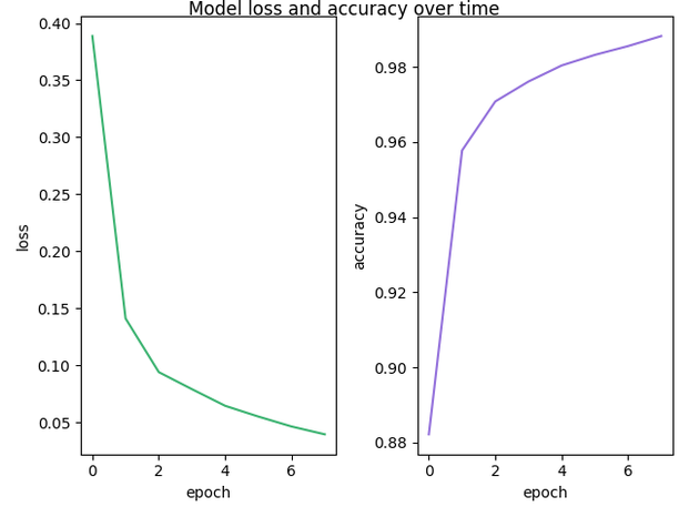
You can see 4 lines in each epoch. Those are our 4 compute nodes. Also, note how the loss and the accuracy are equal for every node – because each node updates the same common variables.
Just to summarize it all together, what this code does is that it sends different batches of the dataset to each of 4 nodes during one epoch. Each node trains the model on a given batch and then aggregates the result in the common variables. All nodes run and train the model in parallel.
Visual representation of loss decreasing and accuracy increasing during the training of the model distributed on 4 nodes:
Results: Comparison of Training Distributed Model on Different Numbers of Nodes
|
Number of nodes |
Code execution time |
Loss |
Accuracy |
|
1 |
393.793 seconds |
0.0041 |
0.9989 |
|
2 |
422.231 seconds |
0.0121 |
0.9968 |
|
3 |
285.436 seconds |
0.0287 |
0.9916 |
|
4 |
209.568 seconds |
0.0397 |
0.9882 |
|
6 |
153.307 seconds |
0.0496 |
0.9845 |
|
8 |
121.635 seconds |
0.0667 |
0.9792 |
|
10 |
101.352 seconds |
0.0849 |
0.9747 |
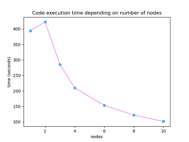
Let’s take a closer look at the table. The most obvious thing about the table is the execution time. We can notice an unexpected behavior at the top of the table: with one and two nodes time starts to increase, but after three nodes time starts to act as expected. The training was run several times, and this behavior is always the same. But what is more important, we can see that with 10 nodes we achieved a significant acceleration of the time! Our time is almost four times better than with one node.
Another thing to notice is the behavior of loss and accuracy metrics of the model. The loss is desired to be as low as possible, and accuracy is desired to be as close to number one as possible. With the increasing of the number of nodes, these values begin to deviate from the desired ones. A simple explanation is that each worker gets a smaller dataset to train the neural network on, so it is logical that precision decreases. Pure statistics! But we should emphasize that these “deviated” values for loss and accuracy are still excellent and in this case still worth the time gain.
You should also be aware of the nodes’ cold start: if nodes are not already allocated by some previous job, they take 1.5 – 2 minutes (on average) to be allocated and to start running the code.
Cleaning Up the Deployment
Log out of theloginnode and let any auto-scaled nodes scale down before deleting the deployment. Delete it by running following command in Google Cloud Shell:
gcloud deployment-manager deployments delete slurm-deployment
Note: slurm-deploymentis our deployment’s name.
Also, check if there are some Slurm images left after deleting the deployment on GCP: Compute Engine → Images.
Click here for part 2 in the series: High Performance Computing with Slurm on AWS

