Iva Marusic
DATA ENGINEER
In previous blog post we had a short introduction to Dataflow SQL and Apache Beam in general, which will be great basis to follow content of this post. We will see which steps are needed to create simple Dataflow SQL job that reads events from Pub/Sub and combines them with data from BigQuery, as well as some additional examples of streaming processing.
Creating first Dataflow SQL job
Throughout this post we will be working with sample data in telco domain: calls and text events, registered on different stations. Stations catalog is stored in BigQuery table, while calls and text events are coming on two different Pub/Sub topics in JSON format.
DATAFLOW SQL UI
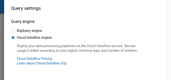
In this first job we will do very simple data enrichment – joining streaming data with data set from BigQuery. All steps will be executed using Console UI, but some of them can be achieved with GCloud commands (query submission). To access Dataflow SQL UI we actually have to navigate to BigQuery UI and change it to use Dataflow engine. This is done by accessingQuery settingsand choosingCloud Dataflow Engine, as seen on picture below.
If you are new to GCP and haven’t used many services, then you might be prompted to enable two APIs: Dataflow and Data Catalog. As mentioned in previous post, Data Catalog is used to store and obtain schema of data sets from sources other than BigQuery. In our case we have 2 different topics, so we will register schemas for them. By default, all topics that exist in GCP project are already registered in Data Catalog, but do not have assigned schema.
Cloud Dataflow Sources
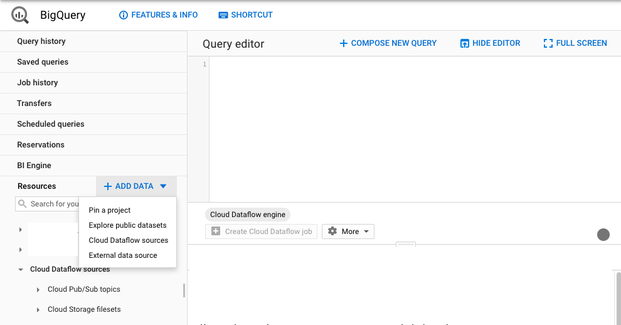
Once we have enabled Dataflow engine in BigQuery, we can notice slight changes of the UI. One additional option is accessible when choosing ADD DATA – Cloud Dataflow sources. All data sets that are used in SQL query need to be registered in BigQuery as Dataflow source. You can choose from Pub/Sub topics and filesets registered in Data Catalog for all projects that you have access to. Since we won’t be working with filesets in this post, how to create fileset in Data Catalog is described here.
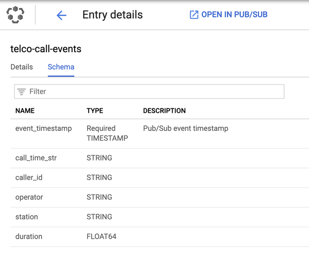
Newly added Dataflow source can be seen listed underCloud Dataflow sourcesinResourcessection in BigQuery console. Having it listed as Dataflow source will allow us to select specific source in query, but we are still missing structure of it. Additional step that needs to be taken is registering schema for added source. In case of Pub/Sub topic, schema is defined directly in BigQuery console, while schema for filesets can be defined in both Data Catalog and BigQuery console. Example schema of call events can be seen on following picture:
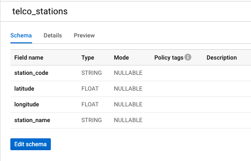
For completeness, this is schema of BigQuery table containing data about stations. Events from Pub/Sub can be joined with table content by comparing station to station_code.
Submitting Dataflow SQL job
Now we are all set for submitting our first Dataflow SQL job by defining a SQL query. We will execute query already seen in part one of this blog sequence:
SELECT calls.*,
stations.station_name AS station_name,
stations.latitude AS station_latitude,
stations.longitude AS station_longitude
FROM pubsub.topic.`project-id`.`telco-call-events` AS calls
LEFT JOIN bigquery.table.`project-id`.dataflow_sql_example.telco_stations AS stations
ON calls.station = stations.station_code;
If there are some mistakes in query syntax or some resources are not defined correctly, query validator will warn us about it. If there are no errors, we can proceed with job creation. Result of this query should have all fields defined in schema of telco-call-events with addition of station_name, latitude and longitude of telco_stations table in BigQuery.
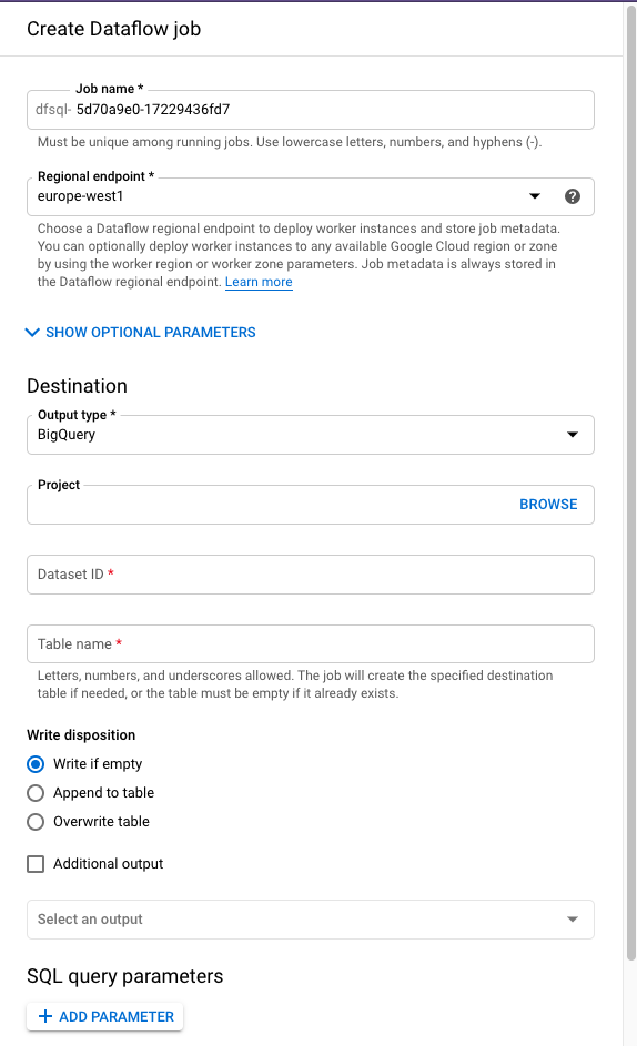
After clicking on Create Cloud Dataflow job button, we are able to define where we want to store the output. At this moment we can choose between BigQuery table (as seen on picture below) or Pub/Sub topic, or both since multiple output destinations are supported. We will store output to BigQuery table that does not exist at the time of job creation. There is no need to create BigQuery table beforehand since schema of output data is known at job creation – defined by SELECT clause in SQL query. Although, if we would like to write data to partition table, we should create it before executing job since there is no option of defining partition field for job.
Besides the output destination, we can define some optional job parameters, such as machine worker type, network and subnetwork. Not all job parameters that can be used in regular Dataflow job are available. To check which parameters are supported visit docs page.
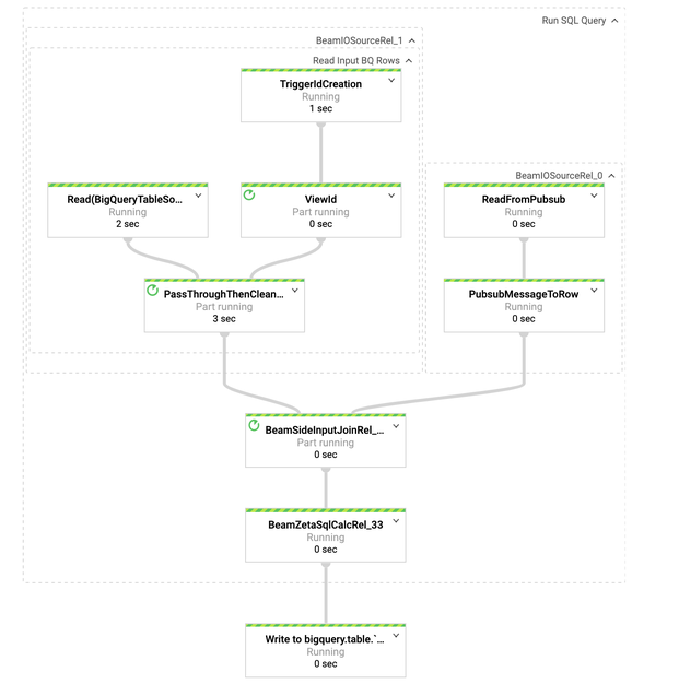
After entering parameters and specifying output destinations, Dataflow SQL job is created by clicking on Create button. It will take a few minutes to construct job graph and spin up worker machines, progress can be checked in logs and Dataflow console. Dataflow job that was constructed based on executed SQL query can be seen on this picture:
This flow is fairly simple and analogy with executed SQL query can be drawn. There are two sources, as defined in FROM clause of SQL query – left source is reading from BigQuery table, while right source is reading from Pub/Sub. Two PCollections are then joined into one and finally written to output BigQuery table.
This concludes our first Dataflow SQL job – we have successfully combined bounded and unbounded collections of data. Steps that were executed can be summarized into following list:
- Add missing Cloud Dataflow sources
- Define schemas for newly added sources
- Construct SQL query
- Define job parameters and output
- Submit Dataflow job
Aggregation of streaming data
So far, we have seen how to perform data enrichment, but we haven’t touched upon real benefit of streaming processing – aggregations and calculations. In out next pipeline we will address that by creating SQL query that groups incoming data and calculates additional metrics.
DEALING WITH UNBOUNDED COLLECTIONS
Since we are dealing with streaming data, grouping is not that easy as when working with bounded collection of data. Collection of data from Pub/Sub is unbounded collection and new elements are constantly being added to pipeline. Grouping on unbounded collection is not possible, since we cannot be sure that we have gathered all elements. To counter that, unbounded collections can be divided using windowing and triggering. Window defines which elements will be logically grouped together based on timestamp assigned to each element. There are different types of windows and triggers, those topics are too broad to be covered in this post. Introduction to windowing and triggers for Apache Beam can be read on their documentation page.
Dataflow SQL offers 3 different types of windows:
· Tumbling windows (called fixed windows in Apache Beam) – represents a consistent, disjoint time interval in the data stream
· Hopping windows (called sliding windows in Apache Beam) – represents a consistent time interval in the data stream, which can overlap
· Session windows – contains elements within agap durationof another element, the gap duration is an interval between new data in a data stream – if data arrives after the gap duration, then data is assigned to a new window.
More about each type of window used in Dataflow SQL, as well as watermark definition and triggers can be found here.
DATAFLOW SQL WITH HOPPING WINDOW
Our next pipeline will be constructed using following query:
SELECT
  HOP_START(“INTERVAL 1 MINUTE”, “INTERVAL 5 MINUTE”) AS period_start,
  HOP_END(“INTERVAL 1 MINUTE”, “INTERVAL 5 MINUTE”) AS period_end,
  calls.station AS station,
  COUNT(calls.caller_id) AS calls_count,
  AVG(calls.duration) AS avg_duration
FROM pubsub.topic.`project-id`.`telco-call-events` AS calls
GROUP BY
  station,
  HOP(calls.event_timestamp, “INTERVAL 1 MINUTE”, “INTERVAL 5 MINUTE”)
We have defined only one input this time, Pub/Sub topic with call events. We will group events by station, calculate number of calls per station (calls_count) and average call duration (avg_duration). As explained in previous section, group per key on its own is not enough – we need to define a window. In this case we have decided to use hopping window that will calculate number of calls and average duration for the last 5 minutes, sliding every 1 minute. What does this mean? It is much easier to understand when looking at an example.
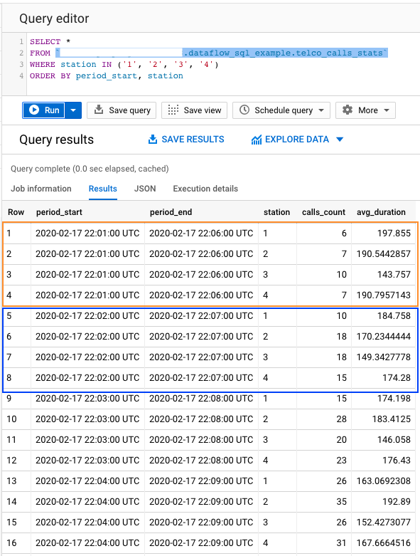
By examining query results, we can notice that difference between period_start and period_end is 5 minutes. First two windows are marked on picture – orange box represents first window, while blue represents second window. We can notice that difference for period_start values of those two windows is 1 minute. These values correspond to our definition of hopping window – calculations are done on 5 minutes of data, with new window beginning every minute. This definition of window also defines overlap of 4 minutes between windows. With a bit of extra knowledge of window functions, we can use common aggregate functions on streaming data, as if we are working with classic tabular data.
Combining multiple unbounded collections
Often there is a need of combining data from different streams in order to do calculations that require certain values from both streams. One such example will be presented in this section.
Last pipeline of this post is defined by following query:
SELECT calls_stream.*,
 sms_stream.sms_count AS sms_count,
 calls_stream.calls_count + sms_stream.sms_count AS events_count
FROM
(
SELECT
   calls.station AS station, COUNT(*) AS calls_count,
   TUMBLE_START("INTERVAL 1 MINUTE") as window_start,
   TUMBLE_END("INTERVAL 1 MINUTE") as window_end
FROM pubsub.topic.`project-id`.`telco-call-events` AS calls
GROUP BY
   calls.station,
   TUMBLE(calls.event_timestamp, "INTERVAL 1 MINUTE")
) AS calls_stream
INNER JOIN
(
SELECT
   sms.station AS station, COUNT(*) as sms_count
FROM pubsub.topic.`project-id`.`telco-sms-events` AS sms
GROUP BY
   sms.station,
   TUMBLE(sms.event_timestamp, "INTERVAL 1 MINUTE")
) as sms_stream
ON
 calls_stream.station = sms_stream.station
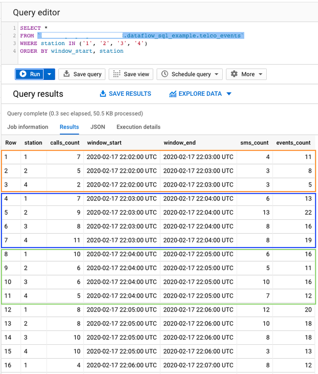
At first, it might look a bit overwhelming, but it is quite simple: we are joining two streams, defined by subqueries, based on station value and calculating events_count as sum of events from both streams. Both subqueries are using windowing to be able to calculate counts of events for certain period. One thing needs to be noticed here: in order for streams to be combinable, they need to have same window definition. We can see that in GROUP clause of both subqueries where tumble window of 1 minute is used. Tumble window is called fixed window in Apache Beam terminology, and it logically groups elements into specific period. For fixed windows there are no overlapping’s, as we can see in picture below.
There are three windows marked on picture – orange box represents first window, blue second, and green third window. We can notice that difference for window_start values of two consecutive windows is 1 minute. Duration of one window is also 1 minute, as it can be seen by comparing window_end and window_start values.
With this example we have shown how streams can be combined to do calculations as data arrives. This allows us to avoid storing data from both streams separately to be able to do any calculations of similar nature. Again, with a bit of more knowledge about window definitions, anyone with experience in SQL can do streaming analytics on multiple streams.
Conclusion
Dataflow SQL makes writing Dataflow pipelines much easier – all you need is SQL knowledge and schema’s assigned to sources. This makes Dataflow accessible to much wider audience and allows data analysts and data scientist to quicker and easier play with new data. Unfortunately, Dataflow SQL lacks some features that are available for standard Dataflow jobs, so it might not be suitable for more complex data pipelines. Since service is relatively new, we should see many more options becoming available in the coming weeks, and months. And we are surely looking forward to them!
Please visit the first part of the blog series:

