Iva Marusic
DATA ENGINEER
n this sequence of blog posts, we will take a look at one of features available on Google Cloud Platform, Dataflow SQL. Recently released in Beta (March 3rd, 2020), Dataflow SQL offers creation of data processing pipelines by simply writing SQL query in BigQuery UI console. First blog post will give introduction to technologies that are backing the Dataflow SQL and compare it to typical Dataflow pipelines.
Dataflow and Apache Beam
Dataflow is the go-to tool on GCP for data processing – fully managed service for unified batch and streaming processing that offers reliable and consistent exactly once processing, horizontal autoscaling of worker resources, flexible resource scheduling (FlexRS) for batch processing, and many other features.
Anyone working on GCP in data domain has most likely come across Dataflow at some point. Some services running on GCP also use Dataflow as their execution engine, for example Cloud Dataprep that executes data transformation recipe as Dataflow job.
Dataflow is in fact one of runners for Apache Beam, open source unified programming model for batch and streaming parallel data processing pipelines. This means that you write your pipelines using Apache Beam SDK and execute them using Dataflow service.
Naturally, if we want to understand Dataflow and use it to its full potential, we first need to look into Apache Beam. Apache Beam offers SDKs for Java, Python and Go (in experimental phase), with addition of SQL in combination with Java – this will be addressed later. Besides Dataflow, you can choose Apache Spark, Apache Flink or any other available runner that supports all features needed by your pipeline. Full list of runners and their capabilities can be found on this link.
APACHE BEAM CORE CONCEPTS
Although main topic of this blog post is not Apache Beam itself, readers need to be at least familiar with core concepts of it to understand the rest of the post.
When designing pipelines, we actually write a Beam driver program with these abstractions of data processing tasks:
Pipeline– encapsulates entire data processing task, from reading input data, transforming it and writing output
PCollection– represents a distributed dataset that is being processed in pipeline, can be bounded (e.g. data from a text file) or unbounded (e.g. messages from Pub/Sub topic)
PTransform– represents a data processing operation, operates on one or more PCollections
I/O transforms– PTransforms that read or write data to various external storage (readers and writers, or sources and sinks)
For more information refer to Apache Beam Programming Guide.
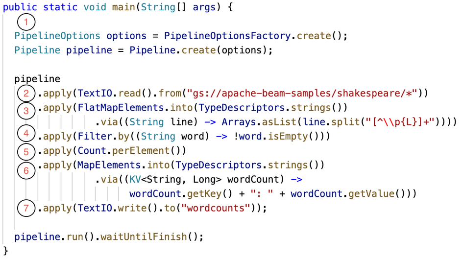
Apache Beam community offers plenty of code examples to get you started. We will take a look at one of the simple pipelines, in two different languages, to get the idea of how the driver program is actually composed. Both code snippets are obtained from and available on Apache Beam GitHub repository.
First picture shows example of Minimal Wordcount pipeline written in Java. For readers that are not familiar with Apache Beam Java syntax, explanation of steps follows:
-
Instance of pipeline is created by providing options that can be passed as program arguments
-
First transformation reads lines from a text file – reader/source transformation that creates first PCollection
-
Each line from file is split into words – output of this step is PCollection of words
-
Filters out words that are empty, leaving only non-empty word in output PCollection
-
Transformation that counts occurrences of same words – output is PCollection of key-value pairs, where key is the word, and value is number of occurrences
-
Key-value pairs are transformed into string representation
-
Results are written to text file – target/sink transformation
With this simple example we can see how the previously explained abstractions are
actually applied. Each transformation is performed by calling apply method, and its
result is used as input for another transformation.
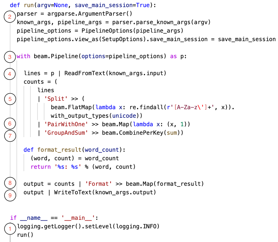
Second example is the same Minimal Word count pipeline but written in Python. There
are some differences in how the pipeline is created and how transformations are called (pipe instead of method call),
but abstractions are the same:
-
Entry point of driver program
-
Creation of options from arguments passed to program (simplified version, check
the original source code for more details) -
Creation of pipeline with pipeline options
-
Transformation that reads lines from text file – reader/source transformation
-
Transformation that applies regex pattern to split lines into words, eliminating
empty words -
For each word we assign it value of one – map phase, output is PCollection of
key-value pairs where key is word and value is 1 -
Transformation that combines same words and produces sum of values – reduce phase,
output is PCollection of key-value pairs where key is word and value is sum of occurrences -
Formats the key-value pairs into strings
-
Writes the result to text file – target/sink transformation
With these two simple examples we can see that there is a bit of coding involved, especially when you need to perform some more complex transformations that are not natively supported by the Apache Beam. To address that issue, we can look into another offering by Apache Beam, Beam SQL.
APACHE BEAM SQL
Apache Beam SQL introduces possibility of querying PCollections using SQL statements. This means that a set of transformation calls can be replaced with single or more SQL queries. Currently it is only available in combination with Beam Java, as you still need to code the pipeline. You can choose between two different SQL dialects: Beam Calcite SQL (variant of Apache Calcite) or Beam ZetaSQL.
In order to support execution of SQL queries, few additional concepts were introduced:
-
SqlTransform – interface for creating PTransforms from SQL statement
-
Row – type of elements that Beam SQL operates on
-
Schema – each PCollection of Row elements needs to have defined schema
How does this work? Each PCollection that is being processed in pipeline needs to contain Row elements, with associated schema. Schema assigns names and value types for each field/column of a row and allows the planner to successfully transform supplied SQL query into set of PTransforms. Planner plays a big role in this setup. It is defined by chosen SQL dialect as SQL query needs to be parsed, evaluated and then turned into a set of PTransforms that produce same result as given SQL statement. Basically, a lot of magic happens under the hood that user does not need to know about.
As an example, we will look into one pipeline that reads data from Pub/Sub and enriches it with additional data from BigQuery table. Messages published to Pub/Sub contain call events (caller id, station from which call was initiated…), while BigQuery table contains details on stations. We will connect station details from BigQuery table with each call record, and store results in separate BigQuery table.
public static void main(String[] args) { BeamExamplePipelineOptions options = PipelineOptionsFactory .fromArgs(args).withValidation().as(BeamExamplePipelineOptions.class); DataflowPipelineOptions dfOptions = options.as(DataflowPipelineOptions.class); Pipeline p = Pipeline.create(dfOptions); Schema callSchema = Schema .builder() .addStringField("call_time_str") .addStringField("caller_id") .addStringField("operator") .addStringField("station") .addDoubleField("duration") .build(); Schema stationSchema = Schema .builder() .addStringField("station_name") .addStringField("station_code") .addDoubleField("longitude") .addDoubleField("latitude") .build(); PCollection callEvents = p .apply("Read PubSubMessages", PubsubIO.readStrings().fromTopic(options.getTopicName())) .apply("PubSubMessage To Row", JsonToRow.withSchema(callSchema)); PCollection stations = p .apply("Read Stations BQ", BigQueryIO.readTableRows().from(options.getInputTable())) .apply("To Row", new BQTableRowToRow()) .setRowSchema(stationSchema); PCollectionTuple callsAndStations = PCollectionTuple .of(new TupleTag<>("CALLS"), callEvents) .and(new TupleTag<>("STATIONS"), stations); PCollection result = callsAndStations .apply("Enrich Data", SqlTransform.query( "SELECT CALLS.*, STATIONS.station_name AS station_name, " + " STATIONS.latitude AS station_latitude, " + " STATIONS.longitude AS station_longitude " + "FROM CALLS " + " LEFT JOIN STATIONS " + " ON CALLS.station = STATIONS.station_code" )); result.apply("To TableRow", ParDo.of(new ToTableRow())) .apply("Write To BQ", BigQueryIO .writeTableRows() .withMethod(BigQueryIO.Write.Method.STREAMING_INSERTS) .withSchema(BigQueryUtils.toTableSchema(result.getSchema())) .withCreateDisposition(BigQueryIO.Write.CreateDisposition.CREATE_IF_NEEDED ) .to(options.getOutputTable()) ); p.run(); }
As previously explained, schemas need to be assigned for each PCollection, in this example we have two: callSchema and stationSchema. There are two collections, each with their corresponding schema: callEvents and stations. Before we are able to apply SQL statement on both collections, we need to “join” them into PCollectionTuple. PCollectionTuple is an abstraction of a map of PCollections, each assigned a unique TupleTag. Once we have defined the PCollectionTuple, we can apply SqlTranform on it. Last step it is to transform the resulting PCollection of Row elements into TableRow elements suitable for BigQuery sink and store the results to BigQuery table. It should be noticed that the schema of result PCollection is automatically resolved from executed query and can be used as input for creation of table in BigQuery.
As reference, this is how the two collections would have been joined in classic Beam Java pipeline:
final PCollectionView<Map<String, Station>> stationsView = stations.apply("Station KV", ParDo.of(new StationKeyValue()).apply(View.asMap());callEvents.apply("Enrich Data", ParDo.of(new DoFn<CallEvent, EnrichedCallEvent>() {@ProcessElementpublic void processElement(ProcessContext c) throws Exception { CallEvent callEvent = c.element(); Map<String, Station> stations = c.sideInput(stationsView); Station station = stations.get(callEvent.station); EnrichedCallEvent ece = new EnrichedCallEvent(); // create instance of EnrichedCallEvent object c.output(ece);}}).withSideInputs(stationsView));
The code snippet above does not have whole pipeline implementation, just the relevant part of it – creation of PCollectionView that is used as a side input to a DoFn implementation that does the enrichment of call events. In this pipeline instead of defining schema we have defined Java model for each input PCollection, including resulting PCollection – something we did not have to do in case of Beam SQL.
Now that we have a rough idea about Apache Beam, Apache Beam SQL and Dataflow, it is time to take a look at Dataflow SQL.
DATAFLOW SQL
Learning yet another programming model or framework can be time consuming and it might take you days/weeks/months before you get your end result. To counter that, Google has already prepared a set of simple pipelines that can be configured and easily deployed in form of Dataflow templates. They have gone one step further and introduced Dataflow SQL as the next step for easier pipeline creation, without the need to code pipelines in Java or Python, or to set up the SDK. The whole process of pipeline creation is done using BigQuery UI in Dataflow SQL mode.
Since you have read through the post up to this point, you might already have an idea how this is implemented in the background. And you probably guessed it, it is done using Apache Beam SQL. Dataflow SQL integrates Beam SQL and supports variant of ZetaSQ Las query syntax which offers better integration with BigQuery resources.
Currently it supports three different sources, Pub/Sub topic, BigQuery table and Cloud Storage filesets, and two targets, Pub/Sub topic and BigQuery table. Since the tool used for pipeline creation is BigQuery UI console, all sources that are being used in pipeline need to accessible in BigQuery. In other words, to be able to use Pub/Sub topic as a source and to reference it in query, we need to add it as Cloud Dataflow source in BigQuery console. Once the sources are added, we need to also define schema for them. This process is very similar to how Apache Beam SQL pipelines are created: for each source PCollection we need to define schema to be able to apply SQL query on them. Once we have everything set up, we are able to write query similar to this:
SELECT calls.*, stations.station_name AS station_name, stations.latitude AS station_latitude, stations.longitude AS station_longitudeFROM pubsub.topic.`project-id`.`telco-call-events` AS callsLEFT JOIN bigquery.table.`project-id`.dataflow_sql_example.telco_stations AS stations ON calls.station = stations.station_code
From hundreds of lines of code, we have reduced pipeline definition to one single SQL query. This query gives same results as Beam SQL pipeline explained in previous section. You might ask, how are the sources created in Beam pipeline? How were the schemas for sources obtained and applied on appropriate source PCollection? Big supporting role in this has Cloud Data Catalog in conjunction with abstraction in Apache Beam calledDataCatalogTableProvider. Sources defined in FROM clause of SQL query are parsed by ZetaSQL query parser that knows which type of source it is. Next step is to obtain schema associated to that source from Data Catalog. The rest of the pipeline is pretty similar to what we have already seen: SQL query is applied as SqlTransform and the results are stored in defined targets defined in pipeline options at job creation time.
For simpler processing tasks Dataflow SQL is the easiest option as it involves minimal amount of coding and it does not require any knowledge of Apache Beam programming model. Every person working in data domain most probably knows SQL well enough and is able to create its custom Dataflow data processing pipeline in matter of hours. The whole process of setting up the Dataflow SQL sources and how jobs are created will be covered in the next blog post. We will also take a look at few different pipelines for data processing with accent on streaming pipelines.
Please visit the second part of the blog series:


