Introduction
Machine learning is a very hot topic in today’s world. From classification, and regression to clustering, we’ve all had some type of encounter with it. Let’s say you don’t have a machine powerful enough to train and test your model, what do you do? We certainly hope you didn’t say that you quit because there are cloud solutions waiting for your models to be trained.
Google Cloud Platform offers specialized AI products but those can be quite expensive. That’s why we here at Syntio developed and tested our own solution based on cloud technologies. In this blog we present to you our take on a topic called “AI in the cloud”. We used our own product, Persistor, to save the data needed for teaching the model, and then wrote some serverless cloud functions that train and test, or make predictions using the AI model.
Why would we do that if there are already enough GCP AI products available out there? That’s a good question with an even better answer. We developed these functions to bring you cheaper solutions for your models. Bear in mind that we are using relatively simple models in this case, so you may find this solution inadequate if your models are more complex.
Our solution will be using CLOUD FUNCTIONS, CLOUD STORAGE, and CLOUD PUB/SUB. Those are billable GCP resources, but we will show you how to effectively use them to help you with your training and testing, and how to save money during that process.
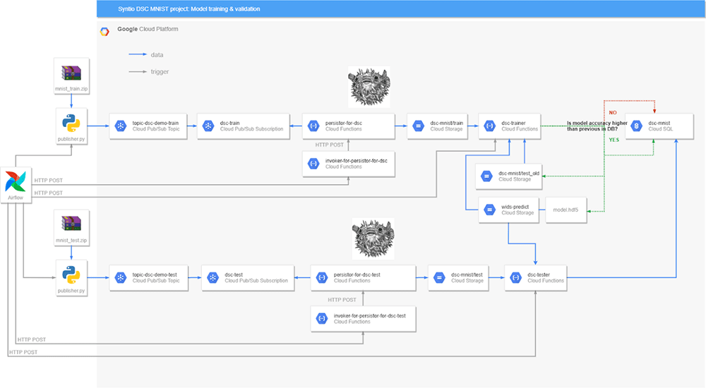
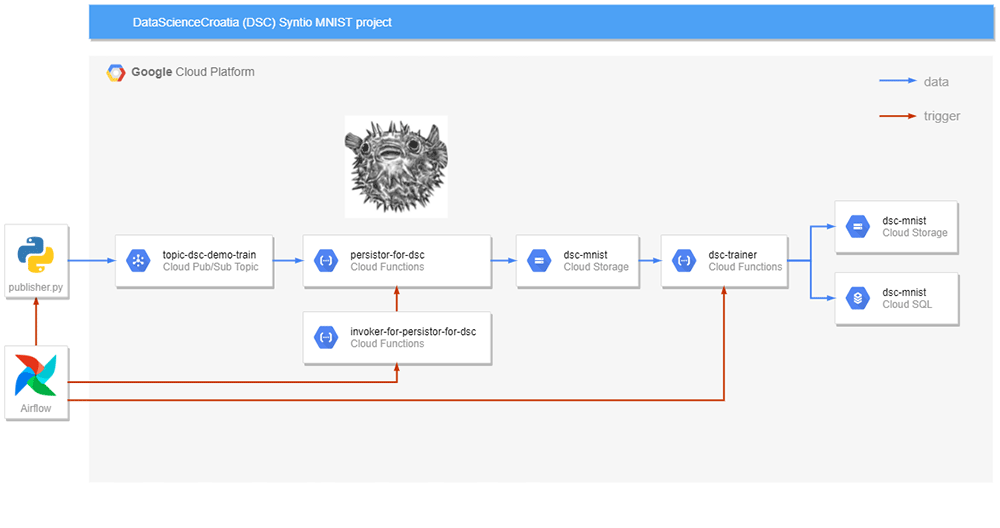
Figure 1 shows the whole architecture of our solution in a very abstract way. We will go into more depth and the step-by-step guide in upcoming sections so don’t worry if you don’t quite get what’s going on right away. We will start by presenting our dataset and the model we used for the solution.
2. MNIST dataset
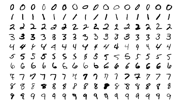
The MNIST (Modified National Institute of Standards and Technology) dataset is a popular large dataset used for training and testing various image processing and machine learning systems. It contains 60,000 training and 10,000 testing images, each containing a handwritten digit. The goal is to have a model which will recognize the digit in the image. You can download the dataset HERE.
Figure 2
We decided to use a Convolutional Neural Network (CNN) model to achieve digit recognition. This approach is very nicely explained in a MEDIUM ARTICLE by Aditi Jain, which we used as a basis for writing our training function.
3. Ingredients on the cheap
Starting at the beginning of our scheme: We will be going from left to right, deep diving into each object shown in the intro section. Let’s dive right in 🙂
3.1 Publisher & Pub/Sub
Figure 3
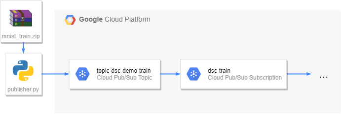
We use the Publisher Python function to publish data read from our dataset. That’s quite literally all there is to it. The Publisher takes data samples from any dataset we feed it (in our example the MNIST dataset) and publishes them to the appropriate topic on the message broker – Cloud PubSub in this case.
The message consists of the unique message ID, metadata, and payload. In our application, the payload is a list of tuples consisting of Base64 encoded images and their respective labels – digits which were drawn onto the image. The list is converted to binary format, which is why it looks like gibberish, but that’s required by Pub/Sub.
Figure 4
Google Cloud Pub/Sub is a message broker that allows services to communicate asynchronously. To put it simply, it saves messages from the senders for as long as it takes the receivers to receive them. Senders or producers of messages are called publishers. Receivers or consumers of those messages are subscribers. Publishers publish messages to topics, and subscribers receive them from subscriptions which are attached to a topic.
3.2 Persistor
Figure 5
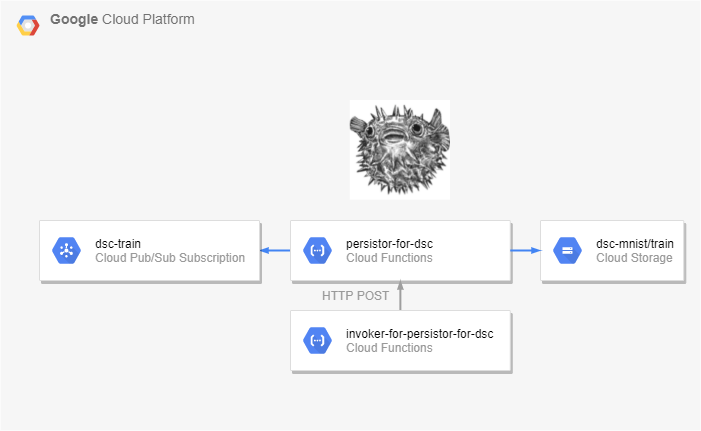
Finally we come to the star of the show PERSISTOR – our product developed for solving data storing issues. You can read more about Persistor on THIS LINK. In this project we used it to back up our data from PubSub to Cloud Storage, which allows us to create multiple models on the same data without needing to publish it again. Persistor is a breeze to install, requires no maintenance, and stores the data in a cheap, accessible way without changing the original data structure. Even better, Persistor is an open source project and you can view and use the source code on its GITHUB page!
3.3 Storage, Functions and SQL
Figure 6
Finally we’ve come to our main logic area. First we’ll explain Cloud Storage and what it’s used for and then we’ll go into depth with Cloud Functions which are our main interest in this blog post (besides Persistor of course).
Google Cloud Storage is an object storage service where you can store any data you’d like. We use it to store our samples and later on, our models. Data is organized into buckets and directories inside them. Persistor takes our samples from the Pub/Sub subscription and stores them in the appropriate storage bucket and directory.
Google Cloud Functions are scalable pay-as-you-go functions as a service (FaaS) that run your code with zero server management. That basically means no virtual machines or containers are needed, and you are only billed for the time your functions run, which makes them pretty cheap. You can customize how many resources the function is given (CPU, RAM) and how long it can run for (maximum timeout is 9 minutes). Cloud functions can be triggered (started) by HTTP requests or events on Cloud Pub/Sub or Cloud Storage.
Cloud SQL is used for storing and managing structured data. It is a fully managed relational database service. We used it with a PostgreSQL database to store our model performance statistics and file usage.
4. The data must flow
Figure 7
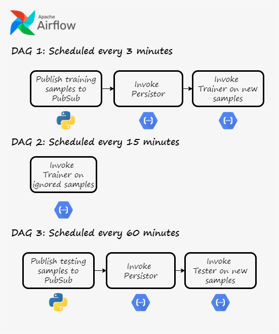
For orchestration we will be using Apache Airflow. It’s going to make sure everything runs smoothly and sequentially. Our version is running locally in a Docker container, but a cloud version is also available on GCP as CLOUD COMPOSER. Airflow enables programming, scheduling, and monitoring workflows. A workflow is represented by a Directed acyclic graph (DAG). Basically, it’s a graph with arrows and without loops
Figure 8
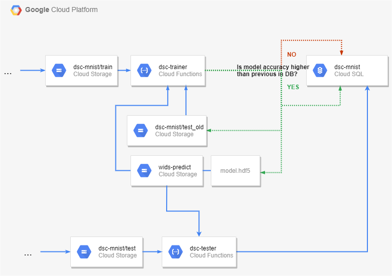
Let’s explain DAG 1. First we process the raw MNIST data in the Publisher function and publish it to a Google Cloud PubSub topic. After that, Airflow triggers our very own Persistor which backs up the messages from PubSub to a Google Cloud Storage bucket. When the Persistor is finished, the Trainer cloud function is triggered. It takes new data from the aforementioned GCS bucket, splits it into training and validation sets, combines new validation samples with used ones, and trains the neural network. If the prediction accuracy is improved, the updated model is saved to GCS along with the validation samples. Model performance is saved to a Cloud SQL database. However, if the accuracy is lower than before, we don’t update the model, but we save the training data for later use. This is where DAG 2 comes into play.
DAG 2 is scheduled to run independently of DAG 1, in wider time intervals. It triggers the Trainer cloud function, but only on ignored data samples – those with which the prediction accuracy did not improve. So, why should we run it again, if it didn’t work the first time? That’s because model performance depends on the grouping of training data. This is the basis for using CROSS VALIDATION techniques.
DAG 3 runs even rarer than DAG 2. The pipeline for acquiring data is identical to the one in the training phase: Pubsub -> Peristor -> Storage. This time, however, we want to use the samples only to test the model we have trained. We achieve this by using the Tester cloud function. It takes our existing trained model, calculates its accuracy using the testing data and saves the accuracy to Cloud SQL.
5. The prediCAKE is ready
Figure 9
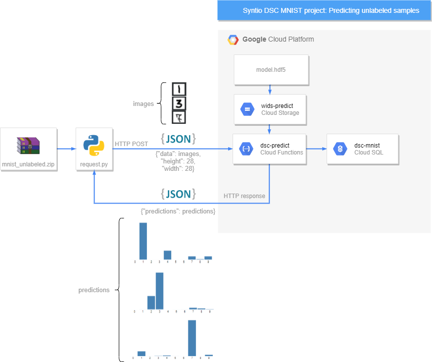
Our finished result is here! We have our model which we can use to predict unlabeled data. Figure 9 shows the whole architecture behind our predicting function. We start by inputting data via a simple Python app which sends HTTP requests to our functions and triggers them that way. HTTP requests are sent with JSON containing encoded images without labels and as a response we get JSON containing an array of predictions for labels.
For one image, we get 10 numbers. Each of them presents the probability of a certain digit being in the image. For example, if we get [0.1, 0.9, 0.2, 0.15, 0.01, 0.05, 0.1, 0.2, 0.1, 0.01], we can conclude that our model thinks that the digit “1” is contained in the image, as the second element in the array has the highest probability (we start counting from 0).
6. Results
Figure 10
On Figure 10 we can see the relationship between model accuracy and the number of samples the model was trained on, as well as the relationship between the value of the loss function and the number of samples. As expected, accuracy increases with the number of samples, and the value of the loss function does that in general, but not always. This is because accuracy is calculated by dividing the number of correctly classified samples with the total number of samples provided for testing, while loss is a little bit more complicated. Basically, it takes into account the probabilities provided by the model for each digit. We could say that when calculating cross entropy loss, we are taking into account exactly how sure the model was in its prediction. Sometimes the model will classify more samples correctly, but it won’t be as sure in those predictions. This is why sometimes we can see both accuracy and loss grow at the same time.
7. Conclusion
By now, some of you probably think all of this is a bit pointless and perhaps overkill. You could train a neural network with the MNIST dataset on your laptop in a matter of minutes, if not less, so why even bother with publishing the dataset, Pub/Sub, Cloud Functions and everything else?
Well, you are right. This is just a proof of concept and on its own it doesn’t make much sense. However, in the real world, we are going to face a much larger amount of data, and it’s often not going to be available all at once. Our dataset could increase over time if we’re dealing with stuff such as social media posts or IoT sensor readings.
The infrastructure for transferring that big data probably already exists, and it consists of applications publishing data to message brokers (sound familiar?). Our project shows how easily you can attach Persistor to that existing data pipeline and leverage Cloud resources not only for data backup, but for very useful analytical purposes, such as machine learning. It’s cheap, efficient, and most importantly: doesn’t require any changes to the existing infrastructure.

